Machine learning, notes 1b: Model selection and validation, the "no free lunch" theorem, and the curse of dimensionality
Now we know a bit about machine learning: it involves models. Machine learning attempts to model data in order to make predictions about the data. In the previous post we dove into the inner functions of a model, and that is very much what machine learning is about. Yet, it’s only half of it, really. The other half has to do with the concept of prediction, and how we make sure our models predict well. This course doesn’t dabble that deep into this other half - but there are a few important topics in this regard that you should be aware of, as they pop up in machine learning all the time.
Model selection and validation
In the previous post, we went over polynomial regression. In the Python implementation, we went with a 4th order polynomial. However, perhaps $M=4$ isn’t the ‘best’ choice for the order of the polynomial - but what is the ‘best’ choice, and how do we find it?
Firstly, the order of our polynomial is set before the training process begins, and we call these special parameters in our model “hyperparameters”. Secondly, the process of figuring out the values of these hyperparameters is called hyperparameter optimization and is a part of model selection. Thirdly, as mentioned in the previous post, machine learning is mostly concerned with prediction, which means that we define the ‘best’ model as the one that generalizes the best on future data, i.e. which model would perform the best on data it wasn’t trained on?
Note that the evaluation metric can be different from the objective function. In fact, it often times is. To figure this out, we usually want to come up with some kind of evaluation metric. Then we divide our training dataset into 3 parts: a training, a validation (sometimes called development), and a test dataset.Commonly the new training dataset is $80\%$ of the original, and the validation and test datasets are $10\%$ each. Then we train our model on the training dataset, perform model selection on the validation dataset, and do a final evaluation of the model on the test dataset. This way, we can determine the model with the lowest generalization error. The generalization error refers to the performance of the model on unseen data, i.e. data that the model hasn’t been trained on.

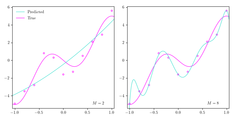
Let’s go back to the polynomial regression example. In the image above I’ve plotted the data points from the previous post together with the true function and $4$ different estimated polynomials of $4$ different orders: $2$, $4$, $6$, and $8$. As we increase the order of the polynomial, we increase what we call the complexity of our model, which roughly can be seen as correlated with the number of parameters in the model. So the more parameters our model has, roughly the more complex it is. As the order of the polynomial (the complexity of the model) increases, it begins approximating the data points better, until it perfectly goes through all the data points. Yet, if we perfectly match the data points in our training dataset, our model probably won’t generalize very well, because the data isn’t perfect; there’s always a bit of noise, which can also be seen above. When we end up fitting our model perfectly to out training dataset, which makes the model generalize poorly, we say that we are overfitting. In the image above, when the order is set to $8$ ($M=8$), we’re definitely overfitting. Conversely, when $M=2$, we could argue that we are underfitting, which means that the complexity of our model isn’t high enough to ‘capture the richness of variation’ in our data. In other words, it doesn’t pick up on the patterns in the data.
Cross-validation
If you have limited data, you might feel disadvantaged with the $80$-$10$-$10$ technique, because the size of the validation and test set is small, thereby not being a proper representation of your entire training set. In the extreme case of only $10$ data points, this would result in a validation and test set of size $1$, which is not exactly a great sample size! Instead, different techniques called cross-validation can be applied. The most common is the k-fold cross-validation technique, where you divide your dataset $\mathcal{D} = \{ \left( \mathbf{x}_1, t_1 \right), \dots, \left(\mathbf{x}_N, t_N \right) \}$ into $k$ distinct subsets. By choosing $1$ of the $k$ subsets to be the validation set, and the rest $k-1$ subsets to be the training set, we can repeat this process $k$ times by choosing a different subset to be the validation set every time. This makes it possible to repeat the training-validation process $k$ times, eventually going through the entire original training set as both training and validation set.
Python implementation
Following the example from last post we can try and figure out the best order $M$ for our polynomial. We start be defining our evaluation metric; we will use the popular mean squared-error (MSE), which is very closely related to the sum of squared errors (SSE) function that we looked at briefly in the last post. The MSE is defined as the mean of the squared differences between our predictions and the true values, formally
\[\text{MSE} = \frac{1}{N} \sum_{n=1}^N \left( t_n - h(x_n,\mathbf{w}) \right)^2,\]The only difference between the mean squared-error and the sum of squared errors is that we’re now dividing by the number of data points.
where $N$ is the number of data points, $h$ is our polynomial, $\mathbf{w}=\left(w_0, \dots, w_M \right)^\intercal$ are the coefficients of our polynomial (the model parameters), and $(x_n, t_n)$ is an input-target variable pair. Below is a simple Python implementation of MSE that takes NumPy arrays as input. Make sure that the true and pred arrays are the same length - this could be done with an assertion if needed.
def mse(true, pred):
    return sum((true-pred)**2) / len(true)
And below is an implementation of k-fold cross-validation. It yields the indices of the train and validation set for each fold. We only have to make sure that n_splits is not larger than n_points.
def kfold(n_points, n_splits=2):
    split_sizes = np.full(n_splits, n_points // n_splits)
    leftover = n_points % n_splits
    split_sizes[:leftover] += 1
    idx = np.arange(n_points)
    current = 0
    for split_size in split_sizes:
        val_idx = idx[current:current+split_size]
        train_idx = np.delete(idx, val_idx)
        yield train_idx, val_idx
        current += split_size
The “no free lunch” theorem
While machine learning tries to come up with the best models, in actuality we empirically choose the best model when confronted with a taskS. Raschka, “Model Evaluation, Model Selection, and Algorithm Selection in Machine Learning,” 2018.. This is what model selection and validation, which we just learned about, does for us. A known theorem in machine learning (and optimization) is the “no free lunch” theoremD. H. Wolpert, “The Lack of A Priori Distinctions Between Learning Algorithms,” 1996., which broadly says that there’s no universally best model. That is, you cannot say that one model is better than another model in all cases, e.g. mixture models are better than neural networks or vice-versa. This is why it’s important to learn about a plethora of models, so when you’re confronted with a task, you know not only to try one model and be content, if it’s doing alright or matches your expectation; there could be another model significantly outperforming, what you’re seeing.
The curse of dimensionality
As mentioned in the beginning, this post is mainly about the issue of determining which models generalize the best. The “no free lunch” theorem tells us that we can never say that one model is the best, and model selection and validation gives us a framework to actually determine the best model for a specific task; the curse of dimensionality is a common enemy in this determination, which is even inherent in our training data! The term was first coined by Richard E. Bellman in 1957R. E. Bellman, “Dynamic Programming,” 1957. to refer to the intractability of certain algorithms in high dimensionality. To facilitate the understanding of the curse of dimensionality, we’ll go through an example of classification. As mentioned in the previous post, classification is a supervised learning task, where we have to organize our data points into discrete groups that we call classes.
So far we’ve been looking at polynomial regression with only a $1$-dimensional input variable $x$. However, in most practical cases, we’ll have to deal with data of high dimensionality, e.g. if humans were our observations, they could have multiple values describing them: height, weight, age, etc. In our example, we’ll have $10$ data points $N=10$, $2$ classes $C=2$, and each data point is $3$-dimensional $D=3$.
import numpy as np

X = np.array([
    [0.33, 0.88, 0.11],
    [0.74, 0.54, 0.62],
    [0.79, 0.07, 0.31],
    [0.83, 0.24, 0.47],
    [0.05, 0.42, 0.47],
    [0.82, 0.70, 0.10],
    [0.51, 0.76, 0.51],
    [0.71, 0.92, 0.59],
    [0.78, 0.19, 0.05],
    [0.43, 0.53, 0.53]
])
t = np.array([0, 0, 0, 0, 0, 1, 1, 1, 1, 1])
The code snippet above shows our training dataset; X is our $10$ input variables of dimensionality $3$ (we have $3$ features), and t is our target variables, which in this case corresponds to $2$ classes. We can also see that the first $5$ data points belong to class $0$ and the last $5$ to class $1$; we have an equal distribution between our classes. If we plot the points using only the first feature (the first column in X), we get the plot underneath. A naive approach to classify the points would be to split the line into $5$ segments (each of length $0.2$), and then decide to classify all the points in this segment into class $0$ or $1$. In the image underneath I’ve coloured the segments after the classification I would make. With this naive approach we get $3$ mistakes.

But let’s see if we can do better! Using the first $2$ features now gives us a grid (of $0.2$ by $0.2$ tiles) that we can now use for our naive classification model. As shown underneath, we can now classify the points such that we only make $1$ mistake.

If we use all $3$ features, we can classify all the points perfectly, which is illustrated underneath. This is because, we now have $0.2$ by $0.2$ by $0.2$ cubes. From this it might seem like using all $3$ features is better than just using $1$ or $2$, since we’re able to better classify our data points - but this is where the counterintuitive concept of the curse of dimensionality comes in, and I tell you that it’s not better to use all the features.
The issue relates to the proportion of our data points compared to our classification sections; with $1$ feature we had $10$ points and $5$ sections, i.e. $\frac{10}{5}=2$ points per section, with $2$ features we had $\frac{10}{5 \times 5}=0.4$ points per section, and with $3$ features we had $\frac{10}{5 \times 5 \times 5}=0.08$ points per section. As we add more features, the available data points in our feature space become exponentially sparser, which makes it easier to separate the data points. Yet, it’s not because of any pattern in the data, in actuality it’s just the nature of higher dimensional spaces. In fact, the data points I listed were randomly generated from a uniform distribution, so the ‘pattern’ we’re fitting to isn’t actually there at all - it’s a result of the increased dimensionality, which makes the available data points become sparser. Because of this inherent sparsity we end up overfitting, when we add more features to our data. Which means we need more data to avoid sparsity, and that’s the curse of dimensionality: as the number of features increase, our data become sparser, which results in overfitting, and we therefore need more data to avoid it.
The illustration underneath shows the exact thing, we just went over. The 100 points are randomly sampled from increasingly higher multivariate normal distributions and randomly assigned to a class. A hyperplane is found that tries to separate these points. As the dimensionality of the points increase, it becomes easier and easier to separate them. In fact, it’s always possible to perfectly separate N+1 points with N-dimensions.

Blessing of non-uniformity
So how do we avoid getting cursed? Luckily, the blessing of non-uniformityP. Domingos, “A few useful things to know about machine learning,” Communications of the ACM, vol. 55, no. 10, pp. 78-87, 2012. comes to our rescue! In most practical (real-world) scenarios our data are not spread out uniformly, but are instead concentrated in some places, which can nullify the curse of dimensionality a little bit. But what if it really is the curse of dimensionality, when we’re overfitting? There’s not a definitive answer, as it really depends on the dataset, but there is a related one in ten rule of thumb; for every model parameter (roughly feature) we want at least $10$ data points. Some better options fall under the topic of dimensionality reduction, which we will look at later on in the course.
Summary
- Hyperparameters are the parameters in a model that are determined before training the model.
- Model selection refers to the proces of choosing the model that best generalizes.
- Training and validation sets are used to simulate unseen data.
- Overfitting happens when our model performs well on our training dataset but generalizes poorly.
- Underfitting happens when our model performs poorly on both our training dataset and unseen data.
- We can see if our model generalizes well with cross-validation techniques.
- The mean squared-error or MSE is a common evaluation metric.
- The “no free lunch” theorem tells us that there is no best model.
- The more features, the higher risk of overfitting is the curse of dimensionality in a nut shell.
- The blessing of non-uniformity counteracts the curse of dimensionality in most practical scenarios.
- Dimensionality reduction can be a tool to remedy the curse of dimensionality.