As mentioned in notes 3a, generative classifiers model the joint probability distribution of the input and target variables $\text{Pr}(\mathbf{x}, t)$. This means, we would end up with a distribution that could generate (hence the name) new input variables with their respective targets, i.e., we can sample new data points with the joint probability distribution, and we will see how to do that in this post.
As mentioned in notes 1a, in classification the possible values for the target variables are discrete, and we call these possible values “classes”. In notes 2 we went through regression, which in short refers to constructing a function $h( \mathbf{x} )$ from a dataset $\mathbf{X} = \left( (\mathbf{x}_1, t_1), \dots, (\mathbf{x}_N, t_N) \right)$ that yields prediction values $t$ for new values of $\mathbf{x}$. The objective in classification is the same, except the values of $t$ are discrete.
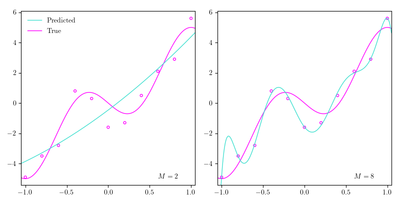
Regression analysis refers to a set of techniques for estimating relationships among variables. This post introduces linear regression augmented by basis functions to enable non-linear adaptation, which lies at the heart of supervised learning, as will be apparent when we turn to classification. Thus, a thorough understanding of this model will be hugely beneficial. We’ll go through 2 derivations of the optimal parameters namely the method of ordinary least squares (OLS), which we briefly looked at in notes 1a, and maximum likelihood estimation (MLE). We’ll also dabble with some Python throughout the post.
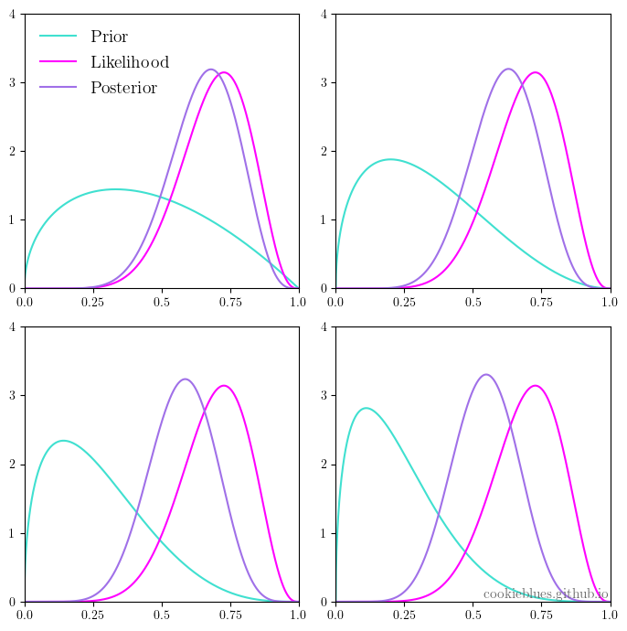
As mentioned in notes 1a, machine learning is mainly concerned with prediction, and as you can imagine, prediction is very much concerned with probability. In this post we are going to look at the two main interpretations of probability: frequentism and Bayesianism.
Now we know a bit about machine learning: it involves models. Machine learning attempts to model data in order to make predictions about the data. In the previous post we dove into the inner functions of a model, and that is very much what machine learning is about. Yet, it’s only half of it, really. The other half has to do with the concept of prediction, and how we make sure our models predict well. This course doesn’t dabble that deep into this other half - but there are a few important topics in this regard that you should be aware of, as they pop up in machine learning all the time.
It seems, most people derive their definition of machine learning from a quote from Arthur Lee Samuel in 1959: “Programming computers to learn from experience should eventually eliminate the need for much of this detailed programming effort.” The interpretation to take away from this is that “machine learning is the field of study that gives computers the ability to learn without being explicitly programmed.”
If you want to work with arrays in Python, you use NumPy. If you want to work with tabular data, you use Pandas. The quintessential Python library for data visualization is Matplotlib. It’s easy to use, flexible, and a lot of other visualization libraries build on the shoulders of Matplotlib. This means that learning Matplotlib will make it easier to understand and work with some of the more fancy visualization libraries.
A friend of mine recently asked me about word embeddings and similarity. I remember, I learned that the typical way of calculating the similarity between a pair of word embeddings is to take the cosine of the angle between their vectors. This measure of similarity makes sense due to the way that these word embeddings are commonly constructed, where each dimension is supposed to represent some sort of semantic meaningThese word embedding techniques have obvious flaws, such as words that are spelled the same way but have different meanings (called homographs), or sarcasm which often times is saying one thing but meaning the opposite.. Yet, my friend asked if you could calculate the correlation between word embeddings as an alternative to cosine similarity, and it turns out that it’s almost the exact same thing.
I recently participated in a challenge orchestrated by Omdena, which (if you don’t already know) is an international hub for AI enthusiasts that want to leverage AI solutions to solve some of humanity’s problems. The challenge was posed by a Nigerian NGO called RA365, and if you want to read more about it, Omdena asked me to write a small article for their blog regarding some work I did in the challenge. I didn’t really do much AI, so I decided to write about just that!
A few people have been asking for a short guide to LaTeX, but since I don’t have that much time on my hands these days, I thought I’d start with a very short guide that I can expand if needed.