Machine learning, notes 1c: Frequentism and Bayesianism
As mentioned in notes 1a, machine learning is mainly concerned with prediction, and as you can imagine, prediction is very much concerned with probability. In this post we are going to look at the two main interpretations of probability: frequentism and Bayesianism.
While the adjective “Bayesian” first appeared around the 1950s by R. A. FisherS. E. Fienberg, “When did Bayesian inference become “Bayesian”?,” 2006., the concept was properly formalized long before by P. S. Laplace in the 18th century, but known as “inverse probability”S. M. Stigler, “The History of Statistics: The Measurement of Uncertainty Before 1900,” ch. 3, 1986.. So while the gist of the Bayesian approach has been known for a while, it hasn’t gained much popularity until recently (last few decades), perhaps mostly due to computational complexity.
The philosophical difference between the frequentist and Bayesian interpretation of probability is their definitions of probability: the frequentist (or classical) definition of probability is based on frequencies of events, whereas the Bayesian definition of probability is based on our knowledge of events. In the context of machine learning, we can interpret this difference as: what the data says versus what we know from the data.
To understand what this means, I like to use this analogy. Imagine you’ve lost your phone somewhere in your home. You use your friend’s phone to call your phone - as it’s calling, your phone starts ringing (it’s not on vibrate). How do you decide, where to look for your phone in your home? The frequentist would use their ears to identify the most likely area from which the sound is coming. However, the Bayesian would also use their ears, but in addition they would recall which areas of their home they’ve previously lost their phone and take it into account, when inferring where to look for the phone. Both the frequentist and the Bayesian use their ears when inferring, where to look for the phone, but the Bayesian also incorporates prior knowledge about the lost phone into their inference.
It’s important to note that there’s nothing stopping the frequentist from also incorporating the prior knowledge in some way. It’s usually more difficult though. The frequentist is really at a loss though, if the event hasn’t happened before and there’s no way to repeat it numerous times. A classic example is predicting if the Arctic ice pack will have melted by some year, which will happen either once or never. Even though it’s not possible to repeat the event numerous times, we do have prior knowledge about the ice cap, and it would be unscientific not to include it.
Bayes’ theorem
Hopefully, these last paragraphs haven’t confused you more than they’ve enlightened, because now we turn to formalizing the Bayesian approach - and to do this, we need to talk about Bayes’ theorem. Let’s say we have two sets of outcomes $\mathcal{A}$ and $\mathcal{B}$ (also called events). We denote the probabilities of each event $\text{Pr}(\mathcal{A})$ and $\text{Pr}(\mathcal{B})$ respectively. The probability of both events is denoted with the joint probability $\text{Pr}(\mathcal{A},\mathcal{B})$, and we can expand this with conditional probabilities
\[\text{Pr}(\mathcal{A},\mathcal{B}) = \text{Pr}(\mathcal{A}|\mathcal{B}) \text{Pr}(\mathcal{B}), \quad \quad (1)\]i.e., the conditional probability of $\mathcal{A}$ given $\mathcal{B}$ and the probability of $\mathcal{B}$ gives us the joint probability of $\mathcal{A}$ and $\mathcal{B}$. It follows that
\[\text{Pr}(\mathcal{A},\mathcal{B}) = \text{Pr}(\mathcal{B}|\mathcal{A}) \text{Pr}(\mathcal{A}) \quad \quad (2)\]as well. Since the left-hand sides of $(1)$ and $(2)$ are the same, we can see that the right-hand sides are equal
\[\begin{aligned} \text{Pr}(\mathcal{A}|\mathcal{B}) \text{Pr}(\mathcal{B}) &= \text{Pr}(\mathcal{B}|\mathcal{A}) \text{Pr}(\mathcal{A}) \\ \text{Pr}(\mathcal{A} | \mathcal{B}) &= \frac{\text{Pr}(\mathcal{B} | \mathcal{A}) \text{Pr}(\mathcal{A})}{\text{Pr}(\mathcal{B})}, \end{aligned}\]which is Bayes’ theorem. This should seem familiar to you - if not, I’d recommend reading up on some basics of probability theory before moving on.
We’re calculating the conditional probability of $\mathcal{A}$ given $\mathcal{B}$ from the conditional probability of $\mathcal{B}$ given $\mathcal{A}$ and the respective probabilities of $\mathcal{A}$ and $\mathcal{B}$. However, it might not be clear-cut, why this is so important in machine learning, so let’s write Bayes’ theorem in a more ‘data sciencey’ way:
\[\overbrace{\text{Pr}(\mathcal{\text{hypothesis}} | \mathcal{\text{data}})}^{\text{posterior}} = \frac{ \overbrace{\text{Pr}(\mathcal{\text{data}} | \mathcal{\text{hypothesis}})}^{\text{likelihood}} \, \overbrace{\text{Pr}(\mathcal{\text{hypothesis}})}^{\text{prior}} }{ \underbrace{\text{Pr}(\mathcal{\text{data}})}_{\text{evidence}} }.\]Usually, we’re not just dealing with probabilities but probability distributions, and the evidence (the denominator above) ensures that the posterior distribution on the left-hand side is a valid probability density and is called the normalizing constantA normalizing constant just ensures that any probability function is a probability density function with total probability of 1.. Since it’s just a normalizing constant though, we often state the theorem in words as
\[\text{posterior} \propto \text{likelihood} \times \text{prior},\]where $\propto$ means “proportional to”.
Example: coin flipping
We’ll start with a simple example that I think nicely illustrates the difference between the frequentist and Bayesian approach. Consider the following problem:
A coin flips heads up with probability $\theta$ and tails with probability $1-\theta$ ($\theta$ is unknown). You flip the coin 11 times, and it ends up heads 8 times. Now, would you bet for or against the event that the next two tosses turn up heads?
For our sake, let’s define some variables. Let $X$ be a random variable representing the coin, where $X=1$ is heads and $X=0$ is tails such that $\text{Pr}(X=1) = \theta$ and $\text{Pr}(X=0) = 1-\theta$. Furthermore, let $\mathcal{D}$ denote our observed data (8 heads, 3 tails). Now, we want to estimate the value of the parameter $\theta$, so that we can calculate the probability of seeing 2 heads in a row. If the probability is less than 0.5, we will bet against seeing 2 heads in a row, but if it’s above 0.5, then we bet for. So let’s look at how the frequentist and Bayesian would estimate $\theta$!
Frequentist approach
As the frequentist, we want to maximize the likelihood, which is to ask the question: what value of $\theta$ will maximize the probability that we got $\mathcal{D}$ given $\theta$, or more formally, we want to find
\[\hat{\theta}_{\text{MLE}} = \underset{\theta}{\arg\max} \text{Pr}(\mathcal{D} | \theta).\]This is called maximum likelihood estimation (MLE). The experiment of flipping the coin 11 times follows a binomial distribution with $n=11$ trials, $k=8$ successes, and $\theta$ the probability of succes. Using the likelihood of a binomial distribution, we can find the value of $\theta$ that maximizes the probability of the data. We therefore want to find the value of $\theta$ that maximizes
\[\text{Pr}(\mathcal{D} | \theta) = \mathcal{L}(\theta | \mathcal{D}) = \begin{pmatrix} 11\\8 \end{pmatrix} \theta^{8} (1-\theta)^{11-8}. \quad \quad (3)\]Note that $(3)$ expresses the likelihood of $\theta$ given $\mathcal{D}$, which is not the same as saying the probability of $\theta$ given $\mathcal{D}$. The image underneath shows our likelihood function $\text{Pr}(\mathcal{D} | \theta)$ (as a function of $\theta$) and the maximum likelihood estimate $\hat{\theta}_{\mathrm{MLE}}$.

Unsurprisingly, the value of $\theta$ that maximizes the likelihood is $\frac{k}{n}$, i.e., the proportion of successes in the trials. The maximum likelihood estimate $\hat{\theta}_{\text{MLE}}$ is therefore $\frac{k}{n} = \frac{8}{11} \approx 0.73$. Assuming the coin flips are independent, we can calculate the probability of seeing 2 heads in a row:
\[\text{Pr}(X=1) \times \text{Pr}(X=1) = \hat{\theta}_{\text{MLE}}^2 = \left( \frac{8}{11} \right)^2 \approx 0.53.\]Since the probability of seeing 2 heads in a row is larger than 0.5, we would bet for!
Bayesian approach
As the Bayesian, we want to maximize the posterior, so we ask the question: what value of $\theta$ will maximize the probability of $\theta$ given $\mathcal{D}$? Formally, we get
\[\hat{\theta}_{\text{MAP}} = \underset{\theta}{\arg\max} \text{Pr}(\theta | \mathcal{D}),\]which is called maximum a posteriori (MAP) estimation. To answer the question, we use Bayes’ theorem
\[\begin{aligned} \hat{\theta}_{\text{MAP}} &= \underset{\theta}{\arg\max} \overbrace{\text{Pr}(\theta | \mathcal{D})}^{\text{posterior}} \\ &= \underset{\theta}{\arg\max} \frac{ \overbrace{\text{Pr}(\mathcal{D} | \theta)}^{\text{likelihood}} \, \overbrace{\text{Pr}(\theta)}^{\text{prior}} }{ \underbrace{\text{Pr}(\mathcal{D})}_{\text{evidence}} }. \end{aligned}\]Since the evidence $\text{Pr}(\mathcal{D})$ is a normalizing constant not dependent on $\theta$, we can ignore it. This now gives us
\[\hat{\theta}_{\text{MAP}} = \underset{\theta}{\arg\max} \text{Pr}(\mathcal{D}|\theta) \, \text{Pr}(\theta).\]During the frequentist approach, we already found the likelihood $(3)$
\[\text{Pr}(\mathcal{D}|\theta) = \begin{pmatrix} 11\\8 \end{pmatrix} \theta^{8} (1-\theta)^{3},\]where we can drop the binomial coefficient, since it’s not dependent on $\theta$. The only thing left is the prior distribution $\text{Pr}(\theta)$. This distribution describes our initial (prior) knowledge of $\theta$. A convenient distribution to choose is the Beta distribution, because it’s defined on the interval [0, 1], and $\theta$ is a probability, which has to be between 0 and 1. Additionally, the Beta distribution is the conjugate prior for the binomial distribution, which broadly means that if the posterior and prior distributions are in the same family, then the prior is the conjugate prior for the likelihood. This is often times a desired property. This gives us
\[\text{Pr}(\theta) = \frac{\Gamma (\alpha) \Gamma (\beta)}{\Gamma (\alpha+\beta)} \theta^{\alpha-1} (1-\theta)^{\beta-1},\]where $\Gamma$ is the Gamma functionThe Gamma function is defined as $\Gamma (n) = (n-1)!$ for any positive integer $n$.. Since the fraction is not dependent on $\theta$, we can ignore it, which gives us
\[\begin{aligned} \text{Pr}(\theta | \mathcal{D}) &\propto \theta^{8} (1-\theta)^{3} \theta^{\alpha-1} (1-\theta)^{\beta-1} \\ &\propto \theta^{\alpha+7} (1-\theta)^{\beta+2}. \quad \quad (4) \end{aligned}\]Note that we end up with another beta distribution (without the normalizing constant).
It is now our job to set the prior distribution in such a way that we incorporate, what we know about $\theta$ prior to seeing the data. Now, we know that coins are usually pretty fair, and if we choose $\alpha = \beta = 2$, we get a beta distribution that favors $\theta=0.5$ more than $\theta = 0$ or $\theta =1$. The illustration below shows this prior $\mathrm{Beta}(2, 2)$, the normalized likelihood, and the resulting posterior distribution.

We can see that the posterior distribution ends up being dragged a little more towards the prior distribution, which makes the MAP estimate a little different the MLE estimate. In fact, we get
\[\hat{\theta}_{\text{MAP}} = \frac{\alpha + k - 1}{\alpha + \beta + n - 2} = \frac{2+8-1}{2+2+11-2} = \frac{9}{13} \approx 0.69,\]which is a little lower than the MLE estimate - and if we now use the MAP estimate to calculate the probability of seeing 2 heads in a row, we find that we will bet against it
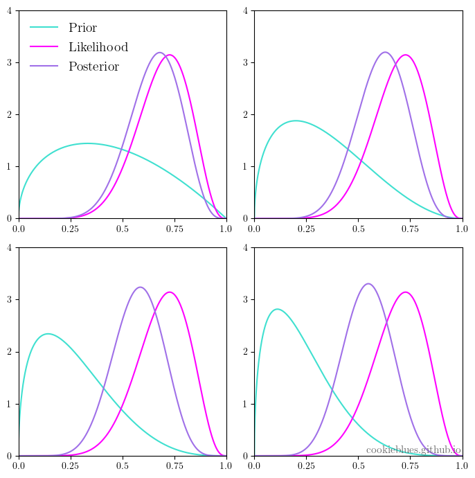
\[\text{Pr}(X=1) \times \text{Pr}(X=1) = \hat{\theta}_{\text{MAP}}^2 = \left( \frac{9}{13} \right)^2 \approx 0.48.\]Furthermore, if we were to choose $\alpha=\beta=1$, we get the special case where the beta distribution is a uniform distribution. In this case, our MAP and MLE estimates are the same, and we make the same bet. The image underneath shows the prior, likelihood, and posterior for different values of $\alpha$ and $\beta$, i.e., for different prior distributions.

Fully Bayesian approach
While we did include a prior distribution in the previous approach, we’re still collapsing the distribution into a point estimate and using that estimate to calculate the probability of 2 heads in a row. However, in a truly Bayesian approach, we wouldn’t do this, as we don’t just have a single estimate of $\theta$ but a whole distribution (the posterior). Let $\mathcal{H}$ denote the event of seeing 2 heads in a row - then we ask: what is the probability of seeing 2 heads given the data, i.e., $\text{Pr}(\mathcal{H} | \mathcal{D})$? To answer this question, we first need to find the normalizing constant for the posterior distribution in $(4)$. Since it’s a beta distribution, we can look at $(4)$ and see that it must be $\frac{\Gamma(\alpha+\beta+11)}{\Gamma(\alpha+8)\Gamma(\beta+3)}$. Like earlier, we’ll also assume that the coin tosses are independent, which means that the probability of seeing 2 heads in a row (given $\theta$ and the data) is just equal to the probability of seeing heads squared, i.e, $\mathrm{Pr} (\mathcal{H} | \theta, \mathcal{D}) = \theta^2$.
We can now answer this question by ‘integrating out’ $\theta$ as
\[\begin{aligned} \mathrm{Pr}(\mathcal{H} | \mathcal{D}) &= \int_{\theta} \mathrm{Pr} (\mathcal{H}, \theta | \mathcal{D}) \, \mathrm{d}\theta \\ &= \int_{\theta} \mathrm{Pr} (\mathcal{H} | \theta, \mathcal{D}) \, \overbrace{\mathrm{Pr} (\theta | \mathcal{D})}^{\mathrm{posterior}} \, \mathrm{d}\theta \\ &= \int_0^1 \theta^2 \, \overbrace{\frac{\Gamma(\alpha+\beta+11)}{\Gamma(\alpha+8)\Gamma(\beta+3)}}^{\text{normalizing constant}} \, \theta^{\alpha+7} (1-\theta)^{\beta+2} \, \mathrm{d}\theta \\ &= \frac{\Gamma(\alpha+\beta+11)}{\Gamma(\alpha+8)\Gamma(\beta+3)} \int_0^1 \theta^{\alpha+9} (1-\theta)^{\beta+2} \, \mathrm{d}\theta \\ &= \frac{\Gamma(\alpha+\beta+11)}{\Gamma(\alpha+8)\Gamma(\beta+3)} \frac{\Gamma(\alpha+10)\Gamma(\beta+3)}{\Gamma(\alpha+\beta+13)} \\ &= \frac{(\alpha+8)(\alpha+9)}{(\alpha+\beta+11)(\alpha+\beta+12)}. \end{aligned}\]In this case, if we choose a uniform prior, i.e., $\alpha=\beta=1$, we actually get $\frac{45}{91} \approx 0.49$, so we would bet against. The reason for this is more complicated and has to do with the uniform prior not being completely agnosticA better choice of prior would be Haldane’s prior, which is the $\mathrm{Beta}(0, 0)$ distribution.. Furthermore, we’ve also made the implicit decision not to update our posterior distribution between the 2 tosses, we’re predicting. You can imagine, we would gain knowledge about the fairness of the coin (i.e., about $\theta$) after tossing the coin the first time, which we could use to update our posterior distribution. However, to simplify the calculations we haven’t done that.